Wrist vs Chest Heart Rate Monitor Accuracy

I usually only wear my Polar GPS watch during my training sessions. I like the simplicity of it, but of course I worry about its accuracy in measuring my heart rate. The watch is good for reporting relative effort between sessions, but now that I’d like to do some heart rate zone based training, is it good enough?

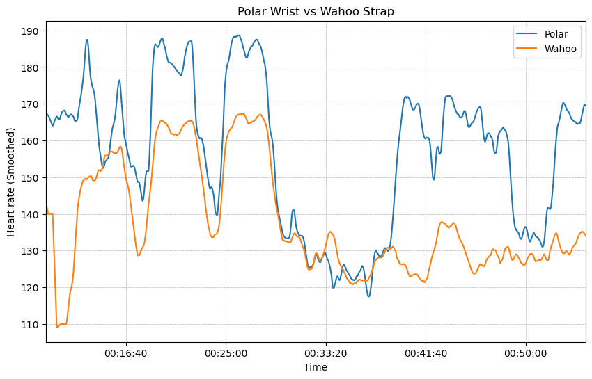
I did an interval training session with my chest strap for comparison purposes. I was a little surprised that the results were so different. Polar states that the wrist measurement is “not necessarily accurate”: What are the pros and cons of different methods for measuring heart rate?

My run consisted of three 4-minute intervals followed by an easy jog. The shape of the curves is similar enough to tell when the intervals occurred, but the watch reports strangely high (incorrect?) heart rates for the easy part of the run. I wonder if this inaccuracy is too bad for training guidance? DCRainmaker has written interesting articles on the same subject: Polar Verity Sense (Optical HR Sensor Band) In-Depth Review (or even the old Troubleshooting your heart rate monitor/strap HR spikes). His results from the different measurement methods seem to be much closer. Why is that? I used the Polar Vantage M and the Wahoo TickrX. And yes, both were worn correctly, i.e. tightly :)

I used the FitParse Python package to parse the HR values from Wahoo’s .fit file. Polar allowed export to .csv so no further parsing was required. Then just some Pandas dataframe and time series mangling to get the data aligned and formatted for creating a graph.

Personal Semantic Search

I have a few thousand notes, a pile of blog posts and tweets, a huge amount of sent emails, and various other data, written by me. In order to get more value out of this dataset, I built a prototype of a personal search engine usgin NLP. I set up a system that automatically connects my emails, notes, posts, chat messages, tweets, book highlights, etc. Now, when writing a new note, I get a list of relevant items written by myself at some earlier time. I think this has a lot of potential for serendipity – at least it’s proven to be amusing.

For example, I wrote some observations about a paper describing how an ML model analysed and graded Airbnb photos: What Makes a Good Image? Airbnb Demand Analytics Leveraging Interpretable Image Features. My system surfaced my old note from 2014 about photography. Very nice! Now I had useful extra context for the new note. Making interesting connections makes data cumulatively better. Both of these notes are now better than they would have been without the connection.

System Structure

First issue to tackle was to somehow import my data from the separate data silos. Then apply some data science methods and use a learning algorithm to distil meaning from the mess. In short:

  1. Import my data from various sources.
  2. Parse through and process the data so that they become indexable documents.
  3. Analyse the documents and build a search index.
  4. Implement a search to the index.

Data Import

I like Karlicoss’s HPI. It’s a concept and an extensible framework for accessing data. The philosophy is to provide a data access layer that abstracts away the trouble of managing multiple data sources with different data models. HPI can import data from APIs, when available, or from local files like the Twitter GDPR export that I used. Note to self: next time I build a service, make sure there’s an API for downloading my data. Written in Python and utilizing namespace packages, HPI allows me to customize and extend to custom data. So I implemented my personal hpi-overlay.

Document Index

For indexing, I tried working with existing tools such as Carrot2 and Solr. The results were not good enough. My main problem was that my data are multi-lingual. A majority is in English, but a lot of data are in other languages: Finnish, German, and French. And by “a lot” I actually mean “a little” because the overall data amounts in my personal space are small from a data science perspective (less than 10.000 documents when excluding emails).

“Traditional” indexing and clustering and making useful searches require some language processing. In order to tokenize and list keywords, we need language-specific stemming. Multiple languages would require multiple setups for stemming, stopwords, etc.

Word Vectors

Instead, I turned to a machine learning algorithm. Fasttext is a word embedding implementation that utilizes subword information. I figured it would be a good candidate to handle a mixed-language dataset, where some languages (Finnish) have high morphology.

I implemented a quick preprocessing tool and exported the texts from all various sources to a single corpus. The resulting corpus size amounted to a mere 12MB. The next step was to train a Fasttext model from scratch, using both subwords and wordNgrams. Training with this multi-language corpus was fast. A quick test using Fasttext’s query tool demonstrated that the model had learned something meaningful. Querying with a misspelled word returned the correct spelling. Querying with a concept returned related concepts. Etc. For example:

Query word?  intelligence
intelligent  0.882046
intellectual 0.778315
artificial   0.777577
episodes     0.724803
treatise     0.714352
terrifying   0.711142
psychology   0.710391
inductive    0.705542
fundamentals 0.703758
visionists   0.701901

The training step could probably be made much better by utilizing pre-trained word vectors and putting more effort in the preprocessing. Cross-lingual embedding space could also prove beneficial for my dataset.

Document Similarity

Now I had a custom model for getting word vectors. Next I took a document, got the vector for each word in the document and created a document vector by averaging the individual word vectors. This is crude approximation and more accurate methods exists, e.g. Le and Mikolov, 2014.

My search index became thus a combination of documents and their correspoding document vectors.

How to find a set of documents that are similar to the one I’m currently working on? Similarity here implies that the documents are somehow related and should be clustered together. Documents are related if they cover the same topic or related topics. For example, are a list of items to pack for a roadtrip related with route planning? Would it be useful to surface both when thinking about the topic?

We have argued that the automated measurement of the similarity between text documents is fundamentally a psychological modeling problem.

Lee corpus

There are multiple potential similarity metrics. See e.g. https://github.com/taki0112/Vector_Similarity for implementation of TS-SS that takes into account vector magnitude and direction. A common and simple similarity metric is to compute the cosine similarity.

For a new note, I would compute the document vector, and then compute cosine similarity with every document vector in the index. As this calculation is done “online” it has a big effect on user experience. I was worried that Python is too slow to be usable. My first implementation affirmed that this was indeed the case, but after turning to Pandas/Numpy and implementing a vectorized version of the computation, the delay became negligible.

Conclusion

Our data are typically siloed in different services, and it is hard to link between items. As so many times before, I was again surprised at how much work it took just to build a dataset for a machine learning project. However, the process is now in place, and HPI is helping to keep it going. Another interesting tool is Promnesia.

Learning a Fasttext model from scratch was surprisingly convenient. The process is fast, and the results are useful. Out-of-vocabulary words are handled by subwords information. Working in the word embedding space seems to make the indexing / similarity more semantic instead of just counting keyword frequencies. Word vectors capture meaning, see e.g. the blog post Less Sexism in Finnish.

After using the system for a while, I’ve been pleasantly surprised to find a long-forgotten note/email/message related to something I’m working on. These reminders from the past have felt useful in making connetions between concepts and building understanding.
Predicate Logic Solving: TPTP vs SMT

Many interesting problems can be presented declaratively using predicate logic. Real life examples are scheduling, logistics, and software and electric circuit verification. That is, the problems are hard and logic provides a way to solve them declaratively. Logic solvers take as input the problem declaration and spit out the solution to the problem.

Examples of solvers are the famous Z3 and GKC. Z3 uses SMTLIB language to specify the problem. GKC is from a different family, and uses TPTP language. The languages are quite different and it seems to me that SMT is geared towards propositional logic while TPTP is for predicate logic. I couldn’t find any simple comparison so I made one.

Our toy predicate logic problem is as follows. We have four people: Agnetha, Björn, Benny, and Anni-Frid (“Frida”), and one binary predicate knows(x,y). We know a priori that:

  • knows(Agnetha, Björn), that is, Agnetha knows Björn.
  • knows(Benny, Björn)
  • ∀x∀y(knows(x,y)→knows(y,x))
  • ∀y¬knows(Frida,y)

Can we say for sure that Agnetha doesn’t know Frida? That is, does the logical consequence hold: S ⊨ ¬knows(Agnetha,Frida)? Simple, but how to write the structure in SMTLIB and TPTP?

First TPTP. The syntax fits this kind of problem very nicely and is clear. Runnning: bin/gkc ./abba.tptp

fof(formula1,axiom, (knows(agnetha,bjorn))).
fof(formula2,axiom, (knows(benny,bjorn))).
fof(formula3,axiom, (! [X] : ! [Y] : ((~ knows(X,Y)) | knows(Y,X)))).
fof(formula4,axiom, (! [X] : ~ knows(frida, X))).
% Proof by contradiction
fof(formula5,conjecture, (~ knows(agnetha,frida))).

Next, the same in SMTLIB. Run with bin/z3 -smt2 abba.smt

; https://smtlib.github.io/jSMTLIB/SMTLIBTutorial.pdf
;(set-logic AUFLIA)
(declare-sort A 0) ; A new sort for persons
(declare-fun knows (A A) Bool)
(declare-const agnetha A)
(declare-const bjorn A)
(declare-const benny A)
(declare-const frida A)
(assert (knows agnetha bjorn))
(assert (knows benny bjorn))
(assert (forall ((x A) (y A)) (=> (knows x y) (knows y x))))
(assert (forall ((x A)) (not (knows frida x))))
;(check-sat)
;(get-model)
; assert the negation of the conjecture
(assert(knows agnetha frida))
(check-sat)

There we have it, the same problem solved in both TPTP and SMTLIB.

This is interesting because the solvers are getting really capable nowadays. Geoff Sutcliffe has written a nice piece about Automated Theorem Proving and how it can be utilized to solve age-old problems.

ATP is thus a technology very suited to situations where a clear thinking domain expert can interact with a powerful tool, to solve interesting and deep problems.

Geoff Sutcliffe

Buying the More Expensive Option

After a visit to a bicycle shop I realised that I need to increase my budget. It makes sense to buy the more expensive bike, as it’s more fun, nicer to ride, and I totally need the fancy features, right?

With this premise I was happy to find Olof Hoverfält‘s post about data-supported decision making. In the genius piece, Olof uses his wardrobe as a case-example of the effect of value-vs-cost. Through meticulous data collection over three years (and counting) he is able to make informed statements about clothing categories, quality, pricing, value, cost of preference, and actual frequency of use. The significance of the post is that it explains important concepts of informed decision making in familiar terms and a relatable context.

Let’s take a look at some highlights.

Real cost. Expensive can be cheap and vice-versa. You can’t know the real cost of an item unless you know it all: purchase price, depreciation rate (or lifetime + value at divestment), actual frequency of use, and quality. A pair of shoes may cost a lot, but if they’re used daily during the looong winter and they can take it (durability), they turn out very cost-effective.

Category differences. There may be subtle differences between seemingly similar categories. Every item in knitwear category is available for wearing every day (unrestricted category). Underwear may spend days in wash cycle after use, becoming available after a significant delay (resricted category). Value of investments can’t be compared directly across categories as the competitive attributes are different.

Cost of quality. The definition of quality is not obvious. Durability is a factor, so it makes sense to buy cheap and durable items. But it makes no sense to buy cheap and durable items that are used very rarely. An expensive shirt may not be cost effective but has other attributes: nicer style and cut, better details and materials, etc. There is a cost related to perceived quality, and the cost can be quantified. In Olof’s post, the cost of “fancy shirts” is 500 euros per year.

Value of long term data. You’d think that after a year of daily tracking you’d have a pretty good data set for making informed decisions about something as simple as clothes. Not so: Olof’s analysis after a year is very different from after three years, and the results keep changing as more data flows in. The actual frequency of use may be very different from the estimate. In terms of data the saying holds: The best time to plant a tree is 20 years ago, the second best time is today.

The data collection template is available at https://hoverfalt.github.io/.

Bayesian Data Analysis of Capacity Factor

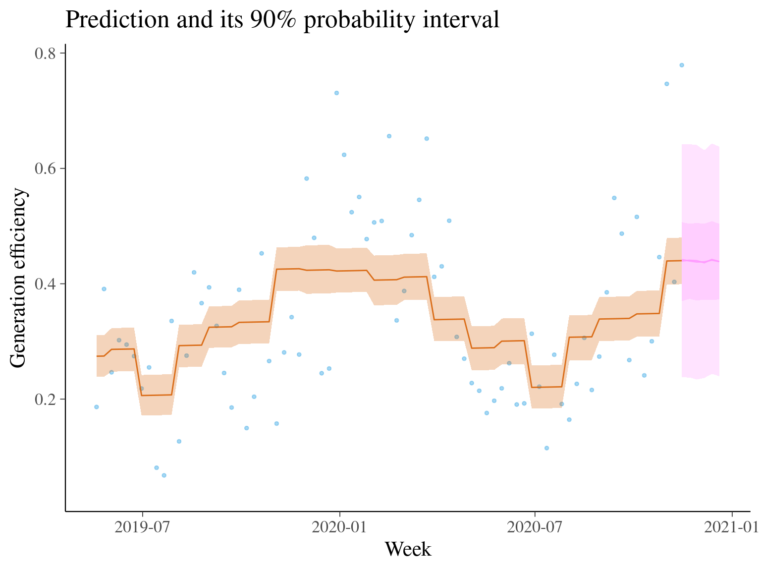
Stan is a platform for probabilistic programming. To demonstrate its features I did data analysis of wind energy capacity factor in Finland. Wind energy is feasible in Finland, and we have quite high seasonal variance, so modeling wind data makes an interesting case. This case study presents a Bayesian data analysis process starting from data, modeling, model diagnostics to conclusions.

Statistical modeling on a modern computing platform such as Stan let’s you construct the model quite freely. I mean, you can all but ignore such constraints as conjugate priors. Stan’s implementation of Hamiltonian Monte Carlo can generate reliable estimates of very hard integrals. You can pay more attention to the model at hand, instead of computational constraints.

The full report is here: Wind Power Generation Efficiency and Seasonality. One reviewer of the report said it well: “In many cases, modeling itself only produces more development ideas than the answers themselves, which is also very evident in this work.”

Original data is from Fingrid (data.fingrid.fi, license CC 4.0 BY).

Covid-19 False Positives

Lab test false positive rates may feel counter-intuitive. Let’s take a closer look at the state-of-the-art Covid-19 real time PCR test.

In Interpreting a covid-19 test result Watson & al., The BJM, May 2020 say that the sensitivity of the test is between 71–98%, and specificity around 95%.

The English statistics authority estimates that in August 2020 about 0.5‰ of the population had the virus. In Finland, THL estimates that there have been a bit under 8000 cases, which would be 1.5‰ of the population. Of these, most are already healed, and the current incidence rate is around 0.03‰ i.e. about a decade better that in England.

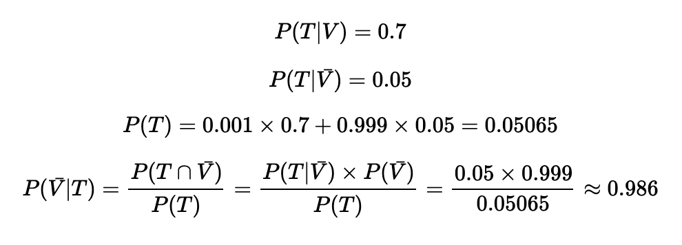
What do the numbers mean in practice? If we pick a random person and the test shows a positive result, what is the probability that the person is actually healthy? Let T = positive test result, and V = has virus. In the BJM article they use sensitivity of 70% for real-life testing. Let’s be generous and say that 1‰ of the population has the virus. Then, according to Bayes’ theorem, we can calculate that there’s a 99% chance the result is a false positive!

How about the opposite case? Pick a random person, test shows negative. What is the probability that the person has the virus anyway? It’s 0.03%.

The key above is the “random person”. The calculations show that there’s no point in testing everyone. In reality, the tested patients are not picked randomly, but they are, and should be, chosen based on their exposure to the virus and/or relevant symptoms.

Functional Programming in Elm—First Impressions

I built a serverless (progressive) web app ppkk.fi using Elm. Elm is a functional language that compiles to JavaScript so you can make web apps and components to use on web sites. Elm is not an extension to JavaScript or something. Indeed, Elm is a stand-alone programming language with its own compiler and standard libraries.

Getting started wasn’t easy. Was the steep learning curve worth it? At this point I’d say it was. A quick list of first impression pros and cons:

Pros

  • When it compiles, it works.
  • Elm-UI makes it possible to avoid complex CSS.
  • Forces good program structure.
  • Pure functions and static types make runtime errors go away.

Cons

  • S l o w to rapidly test new app features. Always have to tie up all loose ends.
  • Have to build up from low level. In JS you’d just npm install a package.

Elm’s pure functions and immutable values forced me to focus on program states, and write functions that are very explicit about the state changes. It was difficult to get right in the beginning. After some UML state diagramming I got the first version running. I quickly realized my first state structure was lacking and started to refactor the code. That was definitely Elm’s strength: refactoring was not the nightmare it often is with e.g. JavaScript. Elm’s compiler checked everything for me, pointed out errors, and I could trust that whenever compiler errors were fixed, I had a pretty solid program up and running again.

For example, I originally had a user data record that was passed to functions building the user interface views. It worked but was difficult with side effects like save to database. So I tagged the data record with a custom type RemoteData that explicitly models writes and loads. With RemoteData User it was nice to build a user interface that doesn’t leave the user wondering if something’s happening or not.

It was even nicer was to find out about phantom types. I could use a phantom type to restrict function parameters to e.g. only “write done” RemoteData User. So now the compiler would check—in compile time—that a function is called with only Users whose data are safe in the database. Proper types and the compilers type checking would help me write an app that would have no runtime errors!

Conclusion: for a simple app Elm was a delightful experience. The result is fast and efficient. I have a feeling tha the code will be reasonable easy to maintain. Specifically, building the user interface with Elm-UI was great. I spent much less than usual time tweaking CSS.

-- 1st version, won't work with side effects
userUpdated : User.Model -> El.Element Msg
userUpdated user = 
  -- ...


-- 2nd version, with remote data
userUpdated : RemoteData User.Model -> El.Element Msg
userUpdated rUser =
  case rUser of
    Loading -> -- Show spinner
    Stored -> -- Show the updated view


-- 3rd version with phantom types
type ValidData a = ValidData
type Loading = Loading
type Saved = Saved

userUpdated : ValidData User.Model -> El.Element Msg
userUpdated validUser =
  user =
    case validUser of
      ValidData u -> u
  -- Now we have a guaranteed valid user record

8 Requirements of Intelligence

What is intelligence, in the context of machine learning and AI? A classic from 1979, Hofstadter’s GEB, gives eight essential abilities for intelligence:

  1. to respond to situations very flexibly
  2. to take advantage of fortuitous circumstances
  3. to make sense out of ambiguous or contradictory messages
  4. to recognize the relative importance of different elements of a situation
  5. to find similarities between situations despite differences which may separate them
  6. to draw distinctions between situations despite similarities which may link them
  7. to synthesize new concept by taking old concepts and putting them together in new ways
  8. to come up with ideas which are novel

It seems to me that the keyword is “flexibility“. Our world is complex, and a creature must be able to act in an infinite variety of circumstances. Sometimes a simple rule is enough, sometimes you need a combination of rules, and sometimes a totally new rule is required.

Hofstadter’s usage of the term stereotyped response got me thinking about Kahneman’s System 1 and 2. In those terms, it seems that System 1 covers all eight abilities. System 1 is fast thinking, applying a stereotypic solution to a situation. No actual reasoning or logical “thinking” is required to fulfil the requirements. However, the stereotypic solutions or rules must be flexible.

Two Views to Zonings Laws

By co-incidence I read two views on zoning. This resonated with me because I haven’t thought about zoning being optional, that is, that there could exist Western cities without proper zoning.

First, about San Francisco:

Imagine you’re searching for an apartment in San Francisco – arguably the most harrowing American city in which to do so. The booming tech sector and tight zoning laws limiting new construction have conspired to make the city just as expensive as New York, and by many accounts more competitive.

Second, about Houston:

Houston is the largest city in the United States without any appreciable zoning. While there is some small measure of zoning in the form of ordinances, deed restrictions, and land use regulations, real estate development in Houston is only constrained by the will and the pocketbook of real estate developers. […] This arrangement has made Houston a very sprawled-out and very automobile-dependent city.

Having lived in the capital area of Finland, that I surmise suffers from a similar effect as San Francisco, I wonder if there are cities that strike the balance right? The housing costs are (too?) high, but I enjoy the beautiful, walkable city.

Visualizing Neural Net Using Occlusion

I got good results using an RNN for a text categorization task. Then I tried using a 1D CNN for the same task. To my surprise, I got even better results, and the model was two magnitudes smaller. How can such a lightweight model perform so well?

Out of curiosity, and also to verify the results, I wanted to visualize what the neural network was learning. This being one-dimensional text data the convolution filter visualizations were not interesting. For image data, check out Understanding Neural Networks Through Deep Visualization.

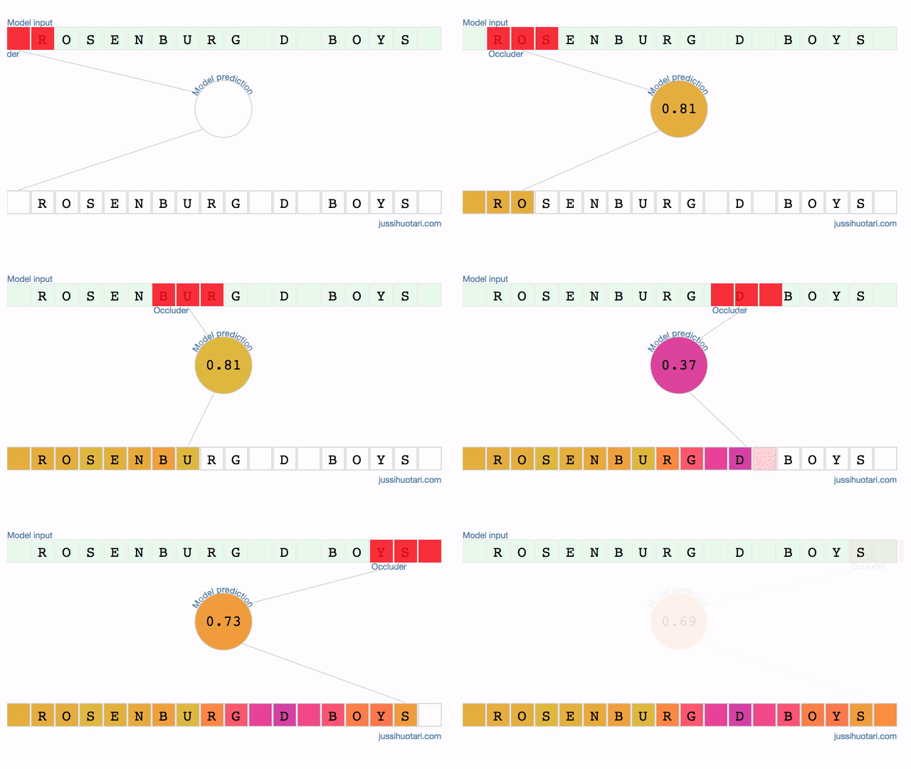
I turned to occlusion, as described in Matthew Zeiler’s paper. To find out what a neural network is recognizing we occlude parts of the input to the network. When the model’s output deviates, the occluded part is significant to the prediction. I haven’t seen occlusion used for text data but decided to give it a go.

Test case: categorize sports team names by age. For example:

 "Westend Old Boys" -> "adult";
 "Indians G Juniors" -> "children";
 "SV Alexanderplatz U7" -> "children";
 "Karlsruhe Erste Männer" -> "adult";

Occlusion Visualization

The model outputs the probability of a junior team. In Finland, D-boys are typically 13-14 years old. When the occluder slides over the characters that signify the age group, i.e. “_D_”, the probability drops drastically. On the other hand, occluding parts of the town name “Rosenburg” makes very little difference. It seems that the model is truly identifying the relevant region in the input data.