I’m working on a text analysis problem and got slightly better results using a CNN than RNN. The CNN is also (much) faster than a recurrent neural net. I wanted to tune it further but had difficulties understanding the Conv1D on the nuts and bolts level. There are multiple great resources explaining 2D convolutions, see for example CS231n Convolutional Neural Networks for Visual Recognition, but I couldn’t find a really simple 1D example. So here it is.
1D Convolution in Numpy
import numpy as np
conv1d_filter = np.array([1,2])
data = np.array([0, 3, 4, 5])
result = []
for i in range(3):
 print(data[i:i+2], "*", conv1d_filter, "=", data[i:i+2] * conv1d_filter)
 result.append(np.sum(data[i:i+2] * conv1d_filter))
print("Conv1d output", result)

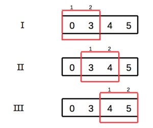
[0 3] * [1 2] = [0  6]
[3 4] * [1 2] = [3  8]
[4 5] * [1 2] = [4 10]

Conv1d output [6, 11, 14]
The input data is four items. The 1D convolution slides a size two window across the data without padding. Thus, the result is an array of three values. In Keras/Tensorflow terminology I believe the input shape is (1, 4, 1) i.e. one sample of four items, each item having one channel (feature). The Convolution1D shape is (2, 1) i.e. one filter of size 2.
The Same 1D Convolution Using Keras
Set up a super simple model with some toy data. The convolution weights are initialized to random values. After fitting, the convolution weights should be the same as above, i.e. [1, 2].
from keras import backend as K
from keras.models import Sequential
from keras.optimizers import Adam
from keras.layers import Convolution1D
K.clear_session()
toyX = np.array([0, 3, 4, 5]).reshape(1,4,1)
toyY = np.array([6, 11, 14]).reshape(1,3,1)

toy = Sequential([
 Convolution1D(filters=1, kernel_size=2, strides=1, padding='valid', use_bias=False, input_shape=(4,1), name='c1d')
])
toy.compile(optimizer=Adam(lr=5e-2), loss='mae')
print("Initial random guess conv weights", toy.layers[0].get_weights()[0].reshape(2,))

Initial random guess conv weights [-0.99698746 -0.00943983]
Fit the model and print out the convolution layer weights on every 20th epoch.
for i in range(200):
  h = toy.fit(toyX, toyY, verbose=0)
  if i%20 == 0:
    print("{:3d} {} \t {}".format(i, toy.layers[0].get_weights()[0][:,0,0], h.history))

  0 [-0.15535446  0.85394686] 	 {'loss': [7.5967063903808594]}
 20 [ 0.84127212  1.85057342] 	 {'loss': [1.288176417350769]}
 40 [ 0.96166265  1.94913495] 	 {'loss': [0.14810483157634735]}
 60 [ 0.9652133   1.96624792] 	 {'loss': [0.21764929592609406]}
 80 [ 0.98313904  1.99099088] 	 {'loss': [0.0096222562715411186]}
100 [ 1.00850654  1.99999714] 	 {'loss': [0.015038172714412212]}
120 [ 1.00420749  1.99828601] 	 {'loss': [0.02622222900390625]}
140 [ 0.99179339  1.9930582 ] 	 {'loss': [0.040729362517595291]}
160 [ 1.00074089  2.00894833] 	 {'loss': [0.019978681579232216]}
180 [ 0.99800795  2.01140881] 	 {'loss': [0.056981723755598068]}
Looks good. The convolution weights gravitate towards the expected values.
1D Convolution and Channels
Let’s add another dimension: ‘channels’. In the beginning this was confusing me. Why is it 1D conv if input data is 2D? In 2D convolutions (e.g. image classification CNN’s) the channels are often R, G, and B values for each pixel. In 1D text case the channels could be e.g. word embedding dimension: a 300-dimensional word embedding would introduce 300 channels in the data and the input shape for single ten words long sentence would be (1, 10, 300).
K.clear_session()
toyX = np.array([[0, 0], [3, 6], [4, 7], [5, 8]]).reshape(1,4,2)
toyy = np.array([30, 57, 67]).reshape(1,3,1)
toy = Sequential([
 Convolution1D(filters=1, kernel_size=2, strides=1, padding='valid', use_bias=False, input_shape=(4,2), name='c1d')
])
toy.compile(optimizer=Adam(lr=5e-2), loss='mae')
print("Initial random guess conv weights", toy.layers[0].get_weights()[0].reshape(4,))

Initial random guess conv weights [-0.08896065 -0.1614058   0.04483104  0.11286306]
And fit the model. We are expecting the weights to be [[1, 3], [2, 4]].
# Expecting [1, 3], [2, 4]
for i in range(200):
  h = toy.fit(toyX, toyy, verbose=0)
  if i%20 == 0:
    print("{:3d} {} \t {}".format(i, toy.layers[0].get_weights()[0].reshape(4,), h.history))

  0 [-0.05175393 -0.12419909  0.08203775  0.15006977] 	 {'loss': [51.270969390869141]}
 20 [ 0.93240339  0.85995835  1.06619513  1.13422716] 	 {'loss': [34.110202789306641]}
 40 [ 1.94146633  1.8690213   2.07525849  2.14329076] 	 {'loss': [16.292699813842773]}
 60 [ 2.87350631  2.8022306   3.02816415  3.09959674] 	 {'loss': [2.602280855178833]}
 80 [ 2.46597505  2.39863443  2.96766996  3.09558153] 	 {'loss': [1.5677350759506226]}
100 [ 2.30635262  2.25579095  3.12806559  3.31454086] 	 {'loss': [0.59721755981445312]}
120 [ 2.15584421  2.15907145  3.18155575  3.42609954] 	 {'loss': [0.39315733313560486]}
140 [ 2.12784624  2.19897866  3.14164758  3.41657996] 	 {'loss': [0.31465086340904236]}
160 [ 2.08049321  2.22739816  3.12482786  3.44010139] 	 {'loss': [0.2942861020565033]}
180 [ 2.0404942   2.26718307  3.09787416  3.45212555] 	 {'loss': [0.28936195373535156]}
...
  n [ 0.61243659  3.15884042  2.47074366  3.76123118] 	 {'loss': [0.0091807050630450249]}
Converges slowly, and looks like it found another fitting solution to the problem.
1D Convolution and Multiple Filters
Another dimension to consider is the number of filters that the conv1d layer will use. Each filter will create a separate output. The neural net should learn to use one filter to recognize edges, another filter to recognize curves, etc. Or that’s what they’ll do in the case of images. This excercise resulted from me thinking that it would be nice to figure out what the filters recognize in the 1D text data.
K.clear_session()
toyX = np.array([0, 3, 4, 5]).reshape(1,4,1)
toyy = np.array([[6, 12], [11, 25], [14, 32]]).reshape(1,3,2)
toy = Sequential([
 Convolution1D(filters=2, kernel_size=2, strides=1, padding='valid', use_bias=False, input_shape=(4,1), name='c1d')
])
toy.compile(optimizer=Adam(lr=5e-2), loss='mae')
print("Initial random guess conv weights", toy.layers[0].get_weights()[0].reshape(4,))

Initial random guess conv weights [-0.67918062  0.06785989 -0.33681798  0.25181985]
After fitting, the convolution weights should be [[1, 2], [3, 4]].
for i in range(200):
  h = toy.fit(toyX, toyy, verbose=0)
  if i%20 == 0:
    print("{:3d} {} \t {}".format(i, toy.layers[0].get_weights()[0][:,0,0], h.history))

  0 [-0.62918061 -0.286818  ] 	 {'loss': [17.549871444702148]}
 20 [ 0.36710593  0.70946872] 	 {'loss': [11.24349308013916]}
 40 [ 1.37513924  1.71750224] 	 {'loss': [4.8558430671691895]}
 60 [ 1.19629359  1.83141077] 	 {'loss': [1.5090690851211548]}
 80 [ 1.00554276  1.95577395] 	 {'loss': [0.55822056531906128]}
100 [ 0.97921425  2.001688  ] 	 {'loss': [0.18904542922973633]}
120 [ 1.01318741  2.00818276] 	 {'loss': [0.064717374742031097]}
140 [ 1.01650512  2.01256871] 	 {'loss': [0.085219539701938629]}
160 [ 0.986902    1.98773074] 	 {'loss': [0.022377887740731239]}
180 [ 0.98553228  1.99929678] 	 {'loss': [0.043018341064453125]}
Okay, looks like first filter weights got pretty close to [1, 2]. How about the 2nd filter?
# Feature 2 weights should be 3 and 4
toy.layers[0].get_weights()[0][:,0,1]

array([ 3.00007081,  3.98896456], dtype=float32)
Okay, looks like the simple excercise worked. Now back to the real work.



 Last Sunday, I read an interesting article in a print magazine. It’s a rare occasion nowadays so I turned back to the story’s first page to find out the writer’s name. Then I opened the